The Basics – Conditional formatting

it’s a lot easier to spot information with color than with anything else. We all know that red is bad, and green is good!
I’m going to show you how conditional formatting can help you and your team in every day documents.

Edit: I just finished a video showing you how to create some conditional formatting:

What is conditional formatting

Well, it’s a tool that formats a cell based on a condition…Often, it is used in finance oriented spreadsheets to show gains and losses. A negative value shows up in red, and a positive value shows up in green.

An excellent tool for tracking

So far, I’ve written a couple articles about data validation and Vlookups. These functions help you save time by streamlining your data entry and by making the document more readable.

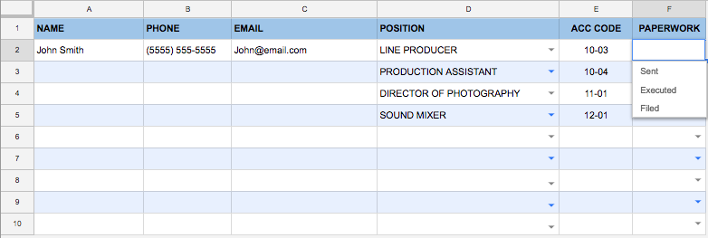
In the crew list that was created for these posts, I’ve added a column to track the paperwork sent to the freelancers listed. It could be anything: W9, start packet, timecard, invoice etc…
I’ve added a drop down using data validation so that my options for this column are:

• Sent
• Executed
• Filed

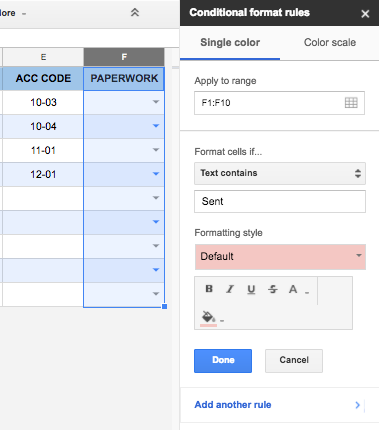
Now, I would like to color code these options. This way, I’ll be reminded of anything sent out but not yet signed. Simply select column F and go to Format > Conditional Formatting.

In the menu that opens in the sidebar, select “Text is exactly” in the drop dow. Then, in the field below, type “Sent” (without quotation marks).

Under Formatting style, select the red background with black text option.

Hit “Done”, and test your formatting rule by selecting “Sent” in one of your cells.

Congratulations, you’ve created your first conditional formatting! Repeat this operation by using the “Add another rule” button. Chose the white background with green text for “Executed” and Green background with black text for “Filed”.

Important note: You can reorganize your rules vertically in the sidebar to prioritize them. Rules at the top override rules under them (if they are triggered by the same conditions).

Formula based condition

The next rule we can set is a little more complex. Ideally, we should be reminded to send out paperwork when a new name is added to the list. If we look at the first entry of our crew list, there are 2 conditions required for this to work:

1. There needs to be some text in cell A2 (the freelancer’s name)
2. Cell F2 needs to be blank (nothing has been done so far)

Select cell F2, open the conditional formatting menu, create a new rule and select “Custom formula is” (all the way at the bottom). The formula we’re going to type in the field will use the following functions:

• “AND( )”, which lets us define that there are multiple arguments to consider
• “ISBLANK( )”, which checks if a cell is blank:
• “NOT( )”, which says that we are looking for the opposite of the data contained in the function

=AND( ISBLANK(F2), NOT( ISBLANK(A2) ) )

In computer speak, this formula says:
“Two conditions: The paperwork cell is empty, and the name cell is not empty”.

Enter this formula in the field, then select the yellow background with black text under formatting style. If you had typed some text in cell F2, remove it. The cell should now be yellow. If you remove the text in cell A2, the cell should be white again.

In order to apply this rule to all the cells in the column, simply copy cell F2, then select column F, go to Edit > Paste special > Paste conditional formatting only.

Conditions can be anything: text, numbers, comparisons etc…It’s also extremely useful to guide users through homemade forms by highliting the cells that need to be filled (“make the cell yellow if blank”).