The Basics – Vlookup

Wouldn’t it be great if the account coding appeared by itself whenever a position is selected in your crew list?

Vlookup is one of excel/google sheet’s most useful formulas. It’s used in many situations, and looks like pure magic if you’re not familiar with it. There are tons of tutorials on how to create a Vlookup, so I’ll explain how to use it in a specific, production oriented case.

Concept

A Vlookup looks through a cell range to find a match to a search key. Once it finds it, the Vlookup can return any value located in a column to the right or our match.

Requirements:
The match to your search key must always be located in the first column of your cell range.
The match will only occur if the search key is identical. If you type a position with a typo, the Vlookup won’t work.

Setup

In a previous post, I explained how to set up data validation in a crew list. This will come in handy, as it will prevent us from making typos.

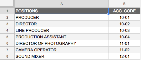I’m going to start by adding account codes to my list of positions.

As you can notice, the first column contains my positions, and the 2nd column contains the codes.

Next, I created a column in my crew list, and labeled it “ACC Code”. Now it’s time to start building the Vlookup.

Syntax

=Vlookup ( search key, cell range, column, FALSE)

Make sure that cell D2 contains a position, then in cell E2, type:

=Vlookup(D2,Positions!A2:B8,2,FALSE)
 note: this only works if the tab with your account codes is called "Positions"

If you did it right, the account code should have magically appeared. the column number (2) refers to the column in the cell range. In our example, column #1 is the list of positions, and column #2 is the account codes.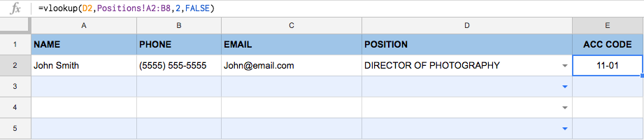

Finishing touches

Because we are going to copy this formula into other rows, we need to make sure the cell range that is being referenced is always the same. Here’s what this looks like:

 =Vlookup(D2,Positions!$A$2:$B$8,2,FALSE)

the $ sign placed in front of a column or row number tells google that these cells are an “absolute” reference (contrary to a “relative” reference). note: this can also be achieved by “naming” the range. More details on named ranges in this post.

Now what happens if there is no position in cell D2? A #N/A error pops up. To avoid that, we can “wrap” our fomula with an “IFERROR” statement.
Note: this only works in google sheets. In excel, you can use something along the lines of “IF(D2<>””,vlookup,””).

IFERROR syntax:
=IFERROR ( the value to return if it’s not an error, the value to return if it is an error)

The 2nd value is even optional. By default IFERROR will return nothing if there is an error.
So, let’s take our Vlookup and wrap it with the IFERROR:

=IFERROR(vlookup(D2,Positions!$A$2:$B$8,2,FALSE))

Formatting issues?

If your accound code just changed to a 5 digit number, it’s because the formatting of the cells in both our positions and crew list tab is off. By default, google sheet or excel will assume that a “00-00” number is a date. We need to tell it it’s actually a custom number. To do that, select the account code column and go to: Format > Number > More formats > Custom number format…

In the field at the top, type: 00-00

Hit apply.

Applying the Vlookup to the other rows

All you need to do to apply this magic trick to the rest of the crew list is copy paste the formula. You’ll notice that when pasting it into cell E3, the formula changed to:

IFERROR(vlookup(D3,Positions!$A$2:$B$8,2,FALSE))

The only thing that changed was the “search key”. Everything else remained the same because we put the $ makers.